
Modeling employee attrition and describing reasons why an employee might quit.
Exploratory Analysis
First, import the data and look at the structure of the variables. There are multiple factors coded as numerics, so I choose to change them all first, then call a summary on the data to get a high-level view of it.
data <- read.csv("/Users/vincentlee/Desktop/UGRID/UGRID2017/HR_analytics.csv")
str(data)
## 'data.frame':    14999 obs. of  10 variables:
##  $ satisfaction_level   : num  0.38 0.8 0.11 0.72 0.37 0.41 0.1 0.92 0.89 0.42 ...
##  $ last_evaluation      : num  0.53 0.86 0.88 0.87 0.52 0.5 0.77 0.85 1 0.53 ...
##  $ number_project       : int  2 5 7 5 2 2 6 5 5 2 ...
##  $ average_montly_hours : int  157 262 272 223 159 153 247 259 224 142 ...
##  $ time_spend_company   : int  3 6 4 5 3 3 4 5 5 3 ...
##  $ Work_accident        : int  0 0 0 0 0 0 0 0 0 0 ...
##  $ left                 : int  1 1 1 1 1 1 1 1 1 1 ...
##  $ promotion_last_5years: int  0 0 0 0 0 0 0 0 0 0 ...
##  $ sales                : Factor w/ 10 levels "accounting","hr",..: 8 8 8 8 8 8 8 8 8 8 ...
##  $ salary               : Factor w/ 3 levels "high","low","medium": 2 3 3 2 2 2 2 2 2 2 ...
data[,3] <- as.factor(data[,3])
data[,5] <- as.factor(data[,5])
data[,6] <- as.factor(data[,6])
data[,7] <- as.factor(data[,7])
data[,8] <- as.factor(data[,8])
str(data)
## 'data.frame':    14999 obs. of  10 variables:
##  $ satisfaction_level   : num  0.38 0.8 0.11 0.72 0.37 0.41 0.1 0.92 0.89 0.42 ...
##  $ last_evaluation      : num  0.53 0.86 0.88 0.87 0.52 0.5 0.77 0.85 1 0.53 ...
##  $ number_project       : Factor w/ 6 levels "2","3","4","5",..: 1 4 6 4 1 1 5 4 4 1 ...
##  $ average_montly_hours : int  157 262 272 223 159 153 247 259 224 142 ...
##  $ time_spend_company   : Factor w/ 8 levels "2","3","4","5",..: 2 5 3 4 2 2 3 4 4 2 ...
##  $ Work_accident        : Factor w/ 2 levels "0","1": 1 1 1 1 1 1 1 1 1 1 ...
##  $ left                 : Factor w/ 2 levels "0","1": 2 2 2 2 2 2 2 2 2 2 ...
##  $ promotion_last_5years: Factor w/ 2 levels "0","1": 1 1 1 1 1 1 1 1 1 1 ...
##  $ sales                : Factor w/ 10 levels "accounting","hr",..: 8 8 8 8 8 8 8 8 8 8 ...
##  $ salary               : Factor w/ 3 levels "high","low","medium": 2 3 3 2 2 2 2 2 2 2 ...
summary(data)
##  satisfaction_level last_evaluation  number_project average_montly_hours
##  Min.   :0.0900     Min.   :0.3600   2:2388         Min.   : 96.0
##  1st Qu.:0.4400     1st Qu.:0.5600   3:4055         1st Qu.:156.0
##  Median :0.6400     Median :0.7200   4:4365         Median :200.0
##  Mean   :0.6128     Mean   :0.7161   5:2761         Mean   :201.1
##  3rd Qu.:0.8200     3rd Qu.:0.8700   6:1174         3rd Qu.:245.0
##  Max.   :1.0000     Max.   :1.0000   7: 256         Max.   :310.0
##
##  time_spend_company Work_accident left      promotion_last_5years
##  3      :6443       0:12830       0:11428   0:14680
##  2      :3244       1: 2169       1: 3571   1:  319
##  4      :2557
##  5      :1473
##  6      : 718
##  10     : 214
##  (Other): 350
##          sales         salary
##  sales      :4140   high  :1237
##  technical  :2720   low   :7316
##  support    :2229   medium:6446
##  IT         :1227
##  product_mng: 902
##  marketing  : 858
##  (Other)    :2923
There are no NAs, and no extreme outliers that suggest false data. Let’s continue by splitting the data between those who left and those who stayed, then comparing the summaries to get a sense of what might differentiate the employees who quit.
library(dplyr)
left <- subset(data, left == 1)
stay <- subset(data, left == 0)
summary(left)
##  satisfaction_level last_evaluation  number_project average_montly_hours
##  Min.   :0.0900     Min.   :0.4500   2:1567         Min.   :126.0
##  1st Qu.:0.1300     1st Qu.:0.5200   3:  72         1st Qu.:146.0
##  Median :0.4100     Median :0.7900   4: 409         Median :224.0
##  Mean   :0.4401     Mean   :0.7181   5: 612         Mean   :207.4
##  3rd Qu.:0.7300     3rd Qu.:0.9000   6: 655         3rd Qu.:262.0
##  Max.   :0.9200     Max.   :1.0000   7: 256         Max.   :310.0
##
##  time_spend_company Work_accident left     promotion_last_5years
##  3      :1586       0:3402        0:   0   0:3552
##  4      : 890       1: 169        1:3571   1:  19
##  5      : 833
##  6      : 209
##  2      :  53
##  7      :   0
##  (Other):   0
##         sales         salary
##  sales     :1014   high  :  82
##  technical : 697   low   :2172
##  support   : 555   medium:1317
##  IT        : 273
##  hr        : 215
##  accounting: 204
##  (Other)   : 613
summary(stay)
##  satisfaction_level last_evaluation  number_project average_montly_hours
##  Min.   :0.1200     Min.   :0.3600   2: 821         Min.   : 96.0
##  1st Qu.:0.5400     1st Qu.:0.5800   3:3983         1st Qu.:162.0
##  Median :0.6900     Median :0.7100   4:3956         Median :198.0
##  Mean   :0.6668     Mean   :0.7155   5:2149         Mean   :199.1
##  3rd Qu.:0.8400     3rd Qu.:0.8500   6: 519         3rd Qu.:238.0
##  Max.   :1.0000     Max.   :1.0000   7:   0         Max.   :287.0
##
##  time_spend_company Work_accident left      promotion_last_5years
##  3      :4857       0:9428        0:11428   0:11128
##  2      :3191       1:2000        1:    0   1:  300
##  4      :1667
##  5      : 640
##  6      : 509
##  10     : 214
##  (Other): 350
##          sales         salary
##  sales      :3126   high  :1155
##  technical  :2023   low   :5144
##  support    :1674   medium:5129
##  IT         : 954
##  product_mng: 704
##  RandD      : 666
##  (Other)    :2281
Some observations:
Those who left had higher monthly hours worked.
Very low level of promotions for those who left. Most high paid employees did not leave.
Those who left had a higher amount of work accidents and ~20% lower satisfaction.
High projects indicates more likely to leave - no one with 7 projects stayed. Since left had higher monthly hours worked, I made a plot to investigate the effect these hours have on the employee’s satisfaction level among those who left, also taking into account number of projects.
library(ggplot2)
ggplot(left, aes(x = average_montly_hours, y = satisfaction_level)) +
  geom_jitter (aes(color = number_project)) +
    labs(title = "Employee Satisfaction vs. Hours Worked", x = "Hours per Month", y = "Satisfaction Level")
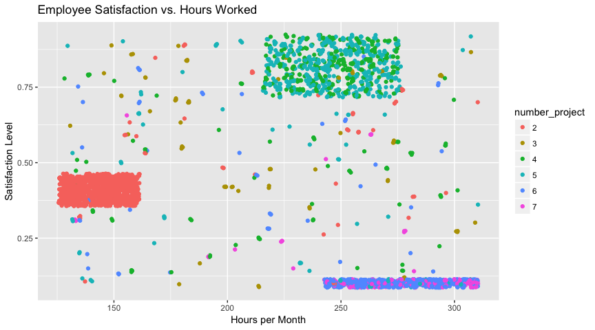
This plot indicates there are three main groups among the employees who quit: those who worked few hours per month and were moderately dissatisfied with their jobs, those who worked normal hours and were moderately-to-very satisfied with their jobs, and those who worked heavy hours who were very dissatisfied with their jobs. Don’t focus on the group that quit while they were satisfied - it is likely due to outside factors like spouse moving or outside promotion. Instead, make conditions better for unsatisfied workers, especially those with many projects and working more than 8 hours a day. Another potential relationship I wanted to explore was between an employee’s satisfaction level and their last evaluation score based on those who left.
ggplot(left, aes(x = last_evaluation, y = satisfaction_level)) + geom_jitter(aes(col = promotion_last_5years)) + labs(title = "Employee Satisfaction from Last Evaluation", x = "Last Evaluation Score", y = "Satisfaction Level")
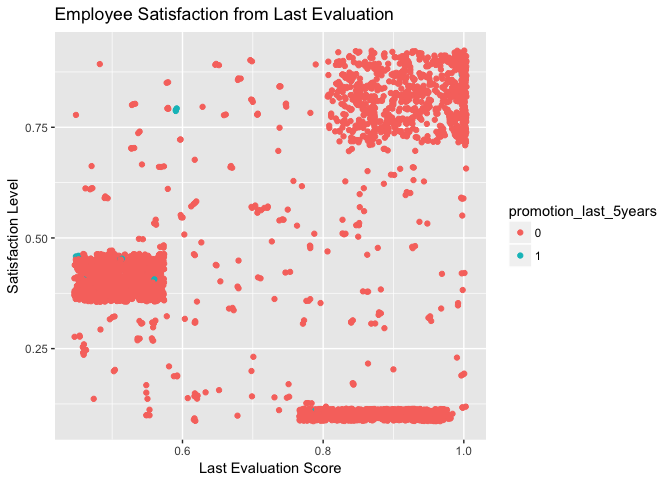
Interestingly, the same clusters emerge: this plot indicates that the same group who works fewer hours are the ones who score low on their evaluation; on the other hand, the ones who work normal-to-heavy schedules all recieved mostly positive evaluations, but are still strongly split between enjoying and hating their jobs. The company needs to avoid assigning people who are already working 9-10 hours a day with more projects in order to keep stress down and satisfaction up. The exceedingly low number of promotions among those who left is also clear in this plot, and perhaps more upward mobility would benefit the company’s employee retention rate.
Modeling
Finally, I wanted to create a model from the data to predict an employee’s satisfaction level. I decided to use linear regression for this task, but I think using logistic regression to predict the variable left could also work well. I started off with a model including all variables, then used stepwise elimination to determine which variables were the most significant towards predicting satisfaction.
modleft <- left[,-7]
mod <- lm(satisfaction_level ~., data = modleft)
step(mod)
mod <- lm(satisfaction_level ~ last_evaluation + number_project +
  average_montly_hours + time_spend_company,
  data = left)
summary(mod)
##
## Call:
## lm(formula = satisfaction_level ~ last_evaluation + number_project +
##     average_montly_hours + time_spend_company, data = left)
##
## Residuals:
##      Min       1Q   Median       3Q      Max
## -0.70806 -0.02640  0.00396  0.03314  0.70992
##
## Coefficients:
##                        Estimate Std. Error t value Pr(>|t|)
## (Intercept)           3.713e-01  2.453e-02  15.132  < 2e-16 ***
## last_evaluation       2.600e-01  2.287e-02  11.369  < 2e-16 ***
## number_project3       1.020e-01  1.634e-02   6.242 4.82e-10 ***
## number_project4       1.382e-01  1.314e-02  10.519  < 2e-16 ***
## number_project5       1.273e-01  1.323e-02   9.626  < 2e-16 ***
## number_project6      -2.906e-01  1.387e-02 -20.948  < 2e-16 ***
## number_project7      -3.048e-01  1.482e-02 -20.558  < 2e-16 ***
## average_montly_hours -3.932e-04  7.316e-05  -5.374 8.18e-08 ***
## time_spend_company3  -3.717e-02  1.782e-02  -2.086   0.0371 *
## time_spend_company4  -9.925e-02  1.625e-02  -6.109 1.11e-09 ***
## time_spend_company5   1.327e-01  1.583e-02   8.386  < 2e-16 ***
## time_spend_company6   1.611e-01  1.713e-02   9.401  < 2e-16 ***
## ---
## Signif. codes:  0 '***' 0.001 '**' 0.01 '*' 0.05 '.' 0.1 ' ' 1
##
## Residual standard error: 0.1071 on 3559 degrees of freedom
## Multiple R-squared:  0.8358, Adjusted R-squared:  0.8353
## F-statistic:  1646 on 11 and 3559 DF,  p-value: < 2.2e-16
anova(mod)
## Analysis of Variance Table
##
## Response: satisfaction_level
##                        Df  Sum Sq Mean Sq  F value    Pr(>F)
## last_evaluation         1   8.264   8.264  720.122 < 2.2e-16 ***
## number_project          5 187.598  37.520 3269.331 < 2.2e-16 ***
## average_montly_hours    1   0.584   0.584   50.881 1.184e-12 ***
## time_spend_company      4  11.399   2.850  248.314 < 2.2e-16 ***
## Residuals            3559  40.844   0.011
## ---
## Signif. codes:  0 '***' 0.001 '**' 0.01 '*' 0.05 '.' 0.1 ' ' 1
The model’s parameters confirm the suspicion that higher number of projects and monthly hours decrease employee satisfaction, and also imply that scoring higher on the last evaluation and loner time spent indicate higher satisfaction, which makes sense. The ANOVA indicates that number of projects and time spent have the highest impact on an employee’s happiness. The model also has a fairly high adjusted R-squared of 0.835, which is much higher than the values when the same model is trained on the stayed (or general) dataset. For some basic diagnostics using ggplot:
library(ggfortify)
autoplot(mod)
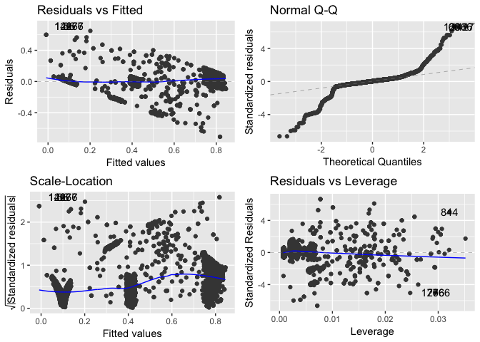
The residuals vs. fitted plot shows that the residuals follow a roughly linear pattern. The Q-Q plot shows the residuals are normally-distributed towards the center, but taper off at the beginning and end. This could potentially be addressed with the use of a transformation term. The scale-location plot shows the model’s lack of equal variance, mostly caused by the three large clusters. The residuals vs. leverage plot shows that no outliers especially affected the model. We can do some basic model fitting to see how well it works to predict the training set.
actual_scores <- left[,1]
pred <- predict(mod, left[,-1], interval="predict")
mse.train <- mean((pred - actual_scores)^2)
mse.train
## [1] 0.04094686
A MSE of only ~0.04% shows that the model can indeed predict the values it has been trained on well, but how about a more general set of data? We can’t use the exact same model because of some missing factor variables in the left subset, but if we retrain the model on all of the data and try another test…
mod <- lm(satisfaction_level ~ last_evaluation + number_project +
  average_montly_hours + time_spend_company,
  data = data)
actual_scores <- data[,1]
pred <- predict(mod, data[,-1], interval="predict")
mse.test <- mean((pred - actual_scores)^2)
mse.test
## [1] 0.1426782
It’s clear the model doesn’t work as well on the more generalized set of data, with a .10 higher MSE.
Conclusions and Next Steps
ggplot(data, aes(x = time_spend_company, y = average_montly_hours, col = left)) + geom_jitter() + labs(title = "Time Spent at Company vs. Average Hours Worked", x = "Years at company", y = "Monthly hours worked")
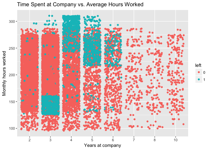
The main cause of employee churn seems to be caused by too many projects being assigned to those already working more than the average amount per week. Spread these out among those who work the least and have the least amount of projects. Try to focus on those who have been working for 3-5 years since the data indicates that these groups are the most likely to quit and the longer an employee stays, the more satisfied and less likely to quit they are.
More advanced modeling could be done to try to predict employee satisfaction or churn. K-means clustering and random forest algorithms could be used to attempt to describe the data. More analysis could also be done into how salary and department may affect churn. Outside variables like how long employees stayed before leaving and more info about their personal lives could help us make better models and more interesting associations among variables.