
For this analysis I chose to examine the relationship between satisfaction level, evaluation score, and the number of projects as indicators of employees leaving. These were found to be the most critical variables in determening employee retention.
Questions:
How to the following factors impact employee retention?
- Employee satisfaction level
- Last evaluation
- Number of projects
- Average monthly hours
- Time spent at the company
- Whether they have had a work accident
- Whether they have had a promotion in the last 5 years
- Department
- Salary
- Whether the employee has left
*This dataset is simulated
Data Summary
library(GGally)
library(ggplot2)
library(dplyr)
##
## Attaching package: 'dplyr'

## The following object is masked from 'package:GGally':
##
##     nasa

## The following objects are masked from 'package:stats':
##
##     filter, lag

## The following objects are masked from 'package:base':
##
##     intersect, setdiff, setequal, union
hrdat = read.csv("/Users/vincentlee/Desktop/UGRID/UGRID2017/HR_analytics.csv")

colnames(hrdat)
##  [1] "satisfaction_level"    "last_evaluation"
##  [3] "number_project"        "average_montly_hours"
##  [5] "time_spend_company"    "Work_accident"
##  [7] "left"                  "promotion_last_5years"
##  [9] "sales"                 "salary"
names(hrdat) = c("sat","eval", "proj", "hrs","years","accident","left","promote","department","salary")


#format as factor variables
hrdat$proj = as.factor(hrdat$proj)
hrdat$years = as.factor(hrdat$years)
hrdat$accident = as.factor(hrdat$accident)
hrdat$promote = as.factor(hrdat$promote)
hrdat$department = as.factor(hrdat$department)
hrdat$salary = as.factor(hrdat$salary)
hrdat$left = as.factor(hrdat$left)

hrdat2 = na.omit(hrdat)

str(hrdat)
## 'data.frame':    14999 obs. of  10 variables:
##  $ sat       : num  0.38 0.8 0.11 0.72 0.37 0.41 0.1 0.92 0.89 0.42 ...
##  $ eval      : num  0.53 0.86 0.88 0.87 0.52 0.5 0.77 0.85 1 0.53 ...
##  $ proj      : Factor w/ 6 levels "2","3","4","5",..: 1 4 6 4 1 1 5 4 4 1 ...
##  $ hrs       : int  157 262 272 223 159 153 247 259 224 142 ...
##  $ years     : Factor w/ 8 levels "2","3","4","5",..: 2 5 3 4 2 2 3 4 4 2 ...
##  $ accident  : Factor w/ 2 levels "0","1": 1 1 1 1 1 1 1 1 1 1 ...
##  $ left      : Factor w/ 2 levels "0","1": 2 2 2 2 2 2 2 2 2 2 ...
##  $ promote   : Factor w/ 2 levels "0","1": 1 1 1 1 1 1 1 1 1 1 ...
##  $ department: Factor w/ 10 levels "accounting","hr",..: 8 8 8 8 8 8 8 8 8 8 ...
##  $ salary    : Factor w/ 3 levels "high","low","medium": 2 3 3 2 2 2 2 2 2 2 ...
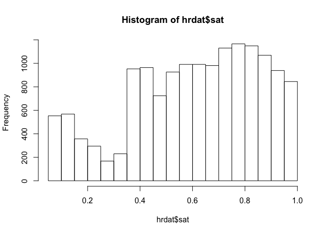
hist(hrdat$sat)
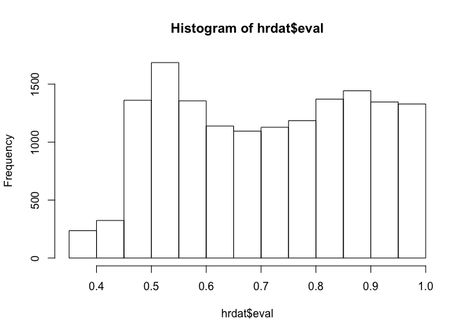
hist(hrdat$eval)
# ggpairs(hrdat)
From this plot of the distribution of evaluation scores, we can see there is a steep drop off at around eval = 0.3. What factors are associated with the sudden jump?
Exploratory Plots
#create exploratory plots
p0 = ggplot(data = hrdat2, aes(salary, fill = proj))
The number of projects is approximately the same between low and medium levels.
p3 = ggplot(data = hrdat, aes(sat, eval, left))
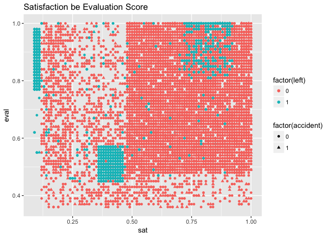
p3 + geom_point(aes(color = factor(left), shape = factor(accident))) + ggtitle("Satisfaction be Evaluation Score")
p3.1 = ggplot(data = hrdat, aes(sat, eval, left))
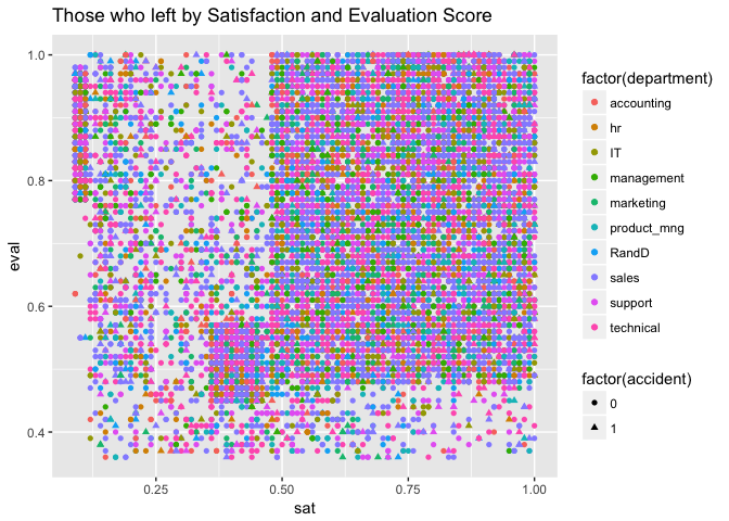
p3.1 + geom_point(aes(color = factor(department), shape = factor(accident))) + ggtitle("Those who left by Satisfaction and Evaluation Score")
p3.1 + geom_point(aes(color = factor(proj))) + ggtitle("Number of Projects, Satisfaction, and Evaluation Score")
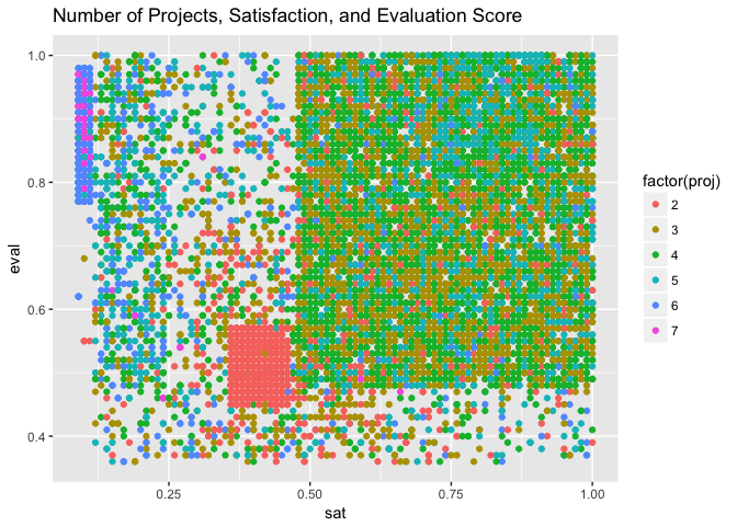 There is clearly some relationship between satisfaction level and evaluation; there are subsets in the population. There doesn’t appear to be a pattern in accidents.
We are interested in the blue box of employees with satisfaction levels from 0.3 to 0.45 and evaluation level 0.3 to 0.5.
The largest determining factor of satisfaction level is the number of projects.
p5 <- ggplot(hrdat, aes(factor(left), sat))

p5 + geom_boxplot(aes(fill = proj))
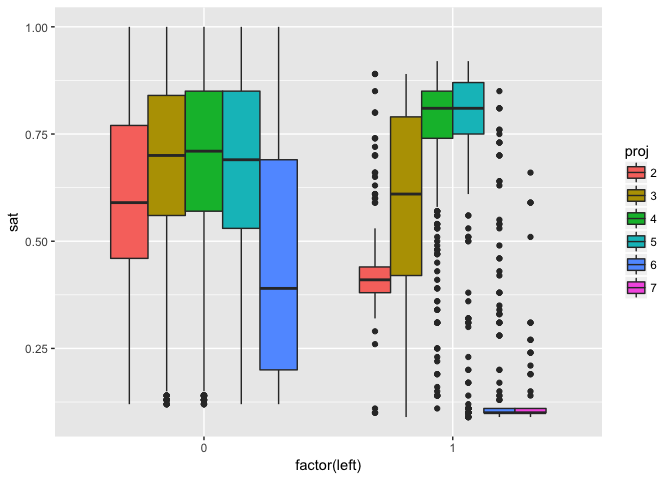 Notice that satisfaction levels at projects 6 and 7 are extremely low. Also notice that no employee with 7 projects stayed, and that satisfaction drops off sharpley with the addition of the 6th project. The blue box on the left shows high variability in those who stay with 6 projects.
Conclusion:
The number of projects appears to be the most powerful predictor of employee retention. The number of work hours should depend on the number of projects. To answer the question on how to best retain employees, we would need to know more about the company stucture. For instance, are employees assigned projects or do they volunteer? What is the skill differential and requirement for different projects? For example, if there are some projects which only a few employees are trained in these specialized topics, they could be getting overloaded. It might be a good idea to examine talent acquisition to ensure that the optimal number of employees are being hired for each type of project.